Robot Painting and Drawing
In this article, ideas and approaches to enable a robot to paint and draw will be proposed and illustrated. Most efforts discussed in this article are applied in the course project of the 10-264 Humanoids (Spring, 2017) class in Carnegie Mellon University.
Problem Formulation
Our team (Aathreya Thuppul, Anni Zhang, David Qiu, Josh Li, Kevan Dodhia and Summer Kitahara) considered building a robot that could paint and draw on different surfaces (canvas, wall, whiteboard, etc.) as our course project based on the Baxter robot platform. We named it the Drawing Baxter project.
For the robot platform we are going to use, the setup is described in Baxter-2, the web page in Dr. Yamaguchi's website.
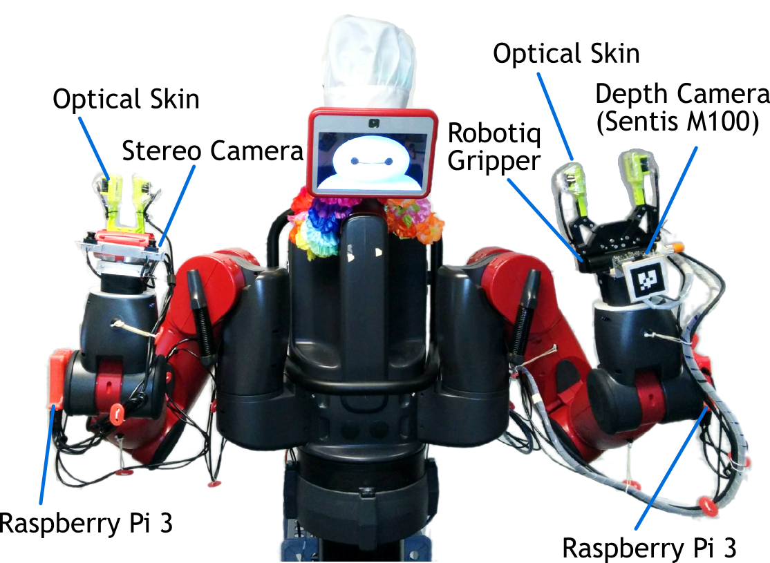
To summarize briefly, it is a Baxter robot with some customized sensors and actuators. The difference between this customized robot platform and the standard Baxter robot platform mainly lies on the two arms of the robot. Both arms are equipped with a Raspberry Pi 3 for lower-level data processing. The left hand of the robot is replaced with a Robotiq Gripper, which yields much stronger output so as to provide larger force when gripping objects. As for the sensors, the left hand is equipped with a Sentis M100 depth camera and the right hand with a pair of stereo cameras. Specially designed sensors, called the Optical Skins, are installed on both the left- and right-hand grippers to provide force feedback.
Our target is to enable the robot to paint and draw on different types of surfaces, such as a wall, a canvas, a whiteboard, and so on. We may design a holder to which we could fix a brush, a pen or a marker, etc. However, it is also plausible that we are going to use the existing grippers on the robot platform to grasp a brush or a marker something directly. How far we go depends on our progress, and our ultimate goal is to enable the robot to paint autonomously with its own creation and draw letters, characters or equations for educational purposes.
Solution Overview
In our short-term plan (proposed at 03/08/2017), we are going to enable the robot to mimic black-white paintings, and learn from experiments to improve our solutions. We are going to let the robot grasp a marker, with its gripper or a customized holder, and paint on a whiteboard. The content we paint is extracted from some black-white images. The solution can be broken up into three parts:
Image content extraction and brushstrokes planning. In this part, an image (currently black-white image, and colored image will be our next step) is uploaded to the robot. A brushstrokes planning algorithm will try to analyse the image and plan brushstrokes so as to recompose the image.
Whiteboard content extraction. In this part, a computer vision program is continuously detecting the position of the whiteboard and extracting the content drawn on it.
Drawing control. In this part, the planned brushtrokes serve as input, which is represented as 2D points in proportional coordinate system of the whiteboard. In a simplified case, all brushstrokes are considered as line segments with thickness, where a pair of 2D points represent the starting and ending points of the brushstrokes. And the purpose of this part is to precisely draw those planned brushstrokes on the whiteboard. Our next steps may include spline from key points and multiple color drawing.
Our plan may alter depending on our progress, and we hope to finally achieve drawing different shapes of brushstrokes in different colors so as to compose colorful pictures fully created by the robot itself. A bonus may be enabling the robot to draw formulas on a whiteboard, which by combining online APIs for solving equations or mathematical problems could serve as a robot that could solve maths and draw the solution process on the whiteboard.
Brushstrokes Planning
The brushstrokes planning algorithm is a gradient-based optimization, which employs the idea of differential dynamic programming (DDP). For more details, one can refer to Dr. Yamaguchi and Prof. Atkeson's 2015 DDP paper and 2016 Graph-DDP paper. To understand the ideas of differential dynamic programming, the Summary for Differential Dynamic Programming with Temporally Decomposed Dynamics may help.
Monochromatic Brushstrokes
To begin with, we are just going to consider planning, or says optimizing, monochromatic brushstrokes. To perform optimization, we need the dynamics model of the canvas for drawing brushstrokes, the reward model and their derivatives. Each brushstroke is considered a dynamics system node. The linear dynamics system consists of multiple nodes in linear structure. Each node $( n_{k} )$ has a state $( \boldsymbol{x}_{k} )$, and an action $( \boldsymbol{a}_{k} )$ is taken after reaching $( \boldsymbol{x}_{n} )$.
In brushstrokes planning, we assume a given black-white target image, and our goal is to plan brushstrokes to draw a picture that maximize the similarity to the target image.
The dynamics model $( F_{k} )$ models the transition from node $( n_{k} )$ to node $( n_{k+1} )$ that
$$ \boldsymbol{x}_{k+1} \leftarrow F_{k} \left( \boldsymbol{x}_{k}, \boldsymbol{a}_{k} \right) $$
where an action are actually a pair of 2D points representing the starting and ending points of a linear brushstroke. And actions are itself the states in this system. However, in the program background, actual images with brushstrokes generated and drawn on it exist to simulate the actual dynamics process, but they will not be considered as states, because it could make the system sophisticated and is not necessary for performing optimization on action sequence. With the simple representation of state and action as a pair of 2D points, the derivative is actually the points themselves to the points themselves, yielding $( 1 )$ or an identical matrix. In other words, the dynamics model derivatives does not alter the shape of the neighbour derivatives in derivative chain rule, instead, it just propagate the original derivatives.
The reward model takes in a state and outputs the corresponding reward that
$$ r_{k} \leftarrow R_{k} \left( \boldsymbol{x}_{k} \right) $$
As discussed in previous paragraph, acutal images are generated in the background to simulate the actual dynamics, so we can track the difference between a previous picture and the next one with a newly drawn brushstroke. The pixels that cover undrawn areas are considered as the contribution of this brushstroke, denoted as $( \triangle_{k} )$. However, the new pixels does not have to be an improvement, which means some of them may cover undesired areas where are kept blank in the target image. So the contribution pixels of a brushstroke can be consider positive, denoted as $( \triangle_{k}^{+} )$, and negative, denoted as $( \triangle_{k}^{-} )$, where it is a constant truth that
$$ \triangle_{k} = \triangle_{k}^{+} + \triangle_{k}^{-} $$
So the exact reward function can be defined as
$$ R_{k} \left( \boldsymbol{x}_{k} \right) = \triangle_{k}^{+} - \triangle_{k}^{-} $$
where proportional coefficients can be added to both terms, thus to define whether not exceeding the border of the target image content or covering more target image content is more important.
As for the derivative of the reward model, we employs a trick, named Computing Gradients by Finite Differences, to approximate the actual value of the reward model derivative. The value of the reward model derivative is approximated by
$$ \frac{ \partial R_{k} \left( \boldsymbol{x}_{k} \right) }{ \partial \boldsymbol{x}_{k} } \approx \frac{ R_{k} \left( \boldsymbol{x}_{k} + \boldsymbol{\epsilon} \right) - R_{k} \left( \boldsymbol{x}_{k} \right) }{ \boldsymbol{\epsilon} } $$
where $( \boldsymbol{\epsilon} )$ is a very small value that add to the difference of the input to yield an approximation of the actual derivative. In the brushstroke planning case, we consider $( \boldsymbol{\epsilon} )$ as a difference value of 3 or 5 pixels something. Here we did not use 1 pixel because the change maybe too small to detect in an accuracy that is limited by the generated pictures. The drawback of using a larger pixel difference is that it may gender unstability at the convergence to boundaries.
With the dynamics model, the reward models and their derivatives, we can now define the value function in Bellman Equation form as
$$ J_{k} \left( \boldsymbol{x}_{k}, \boldsymbol{U}_{k} \right) = R_{k+1} \left( F_{k} \left( \boldsymbol{x}_{k}, \boldsymbol{a}_{k} \right) \right) + \gamma J_{k+1} \left( F_{k} \left( \boldsymbol{x}_{k}, \boldsymbol{a}_{k} \right) \right) $$
where $( \boldsymbol{U}_{k} )$ is the action sequence starting from node $( n_{k} )$ to the last second node $( n_{N-1} )$, and $( \gamma = 1 )$ is assumed in our case.
The derivative of the value function with respect to action is then able to expressed in Bellman Equation form as
$$ \frac{ \partial J_{k} }{ \partial \boldsymbol{a}_{k} } = \frac{ \partial F_{k} }{ \partial \boldsymbol{a}_{k} } \frac{ \partial R_{k+1} }{ \partial \boldsymbol{x}_{k+1} } + \gamma \frac{ \partial F_{k} }{ \partial \boldsymbol{a}_{k} } \frac{ \partial J_{k+1} }{ \partial \boldsymbol{x}_{k+1} } $$
The goal of optimization is to maximize the value function $( J )$ started from the beginning node $( n_{0} )$ with respect to the action sequence $( \boldsymbol{U}_{0} \equiv \left\{ \boldsymbol{a}_{0}, \boldsymbol{a}_{1}, \dots, \boldsymbol{a}_{N-1} \right\} )$, that
$$ \boldsymbol{U}_{0}^{*} \leftarrow \arg\max_{\boldsymbol{U}_{0}} J_{0} \left( \boldsymbol{x}_{0}, \boldsymbol{U}_{0} \right) $$
With the derivative of the value function, we could employ gradient-based optimization method the search for the (locally) optimal action sequene $( \boldsymbol{U}_{0}^{*} )$.
References
- Combining Finger Vision and Optical Tactile Sensing: Reducing and Handling Errors While Cutting Vegetables, A. Yamaguchi and C. G. Atkeson, 2016
- Differential Dynamic Programming with Temporally Decomposed Dynamics, A. Yamaguchi and C. G. Atkeson, 2015
- Differential Dynamic Programming for Graph-Structured Dynamical Systems: Generalization of Pouring Behavior with Different Skills, A. Yamaguchi and C. G. Atkeson, 2016